The Schrödinger Bridge Problem
a dynamical formulation of optimal transport
Introduction
In many problems of the sciences, one core fundamental problem is on optimal transport, which deals with how masses are transported from one to another. One popular application in machine learning is generative modeling, where goal is to generate data from noise. This can be seen as a mass transportation problem where the target distribution (masses) is some data distribution and the initial distribution is Gaussian. Diffusion models are one of the numerous methods proposed motivated by this very idea of optimal transport.
Beyond generative modeling, one could also try to transport one data distribution to another. The goal here is to not only generate high quality samples, but also have certain properties of the coupling, as paired training examples are not necessarily available.
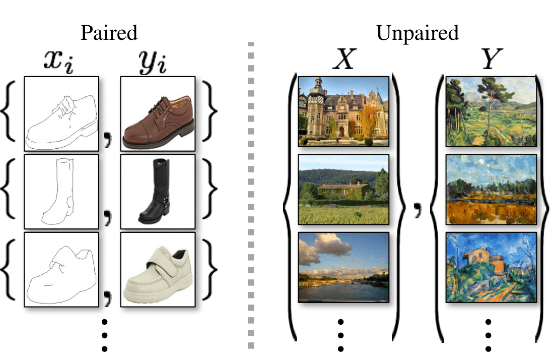
Applications naturally arising from this problem is style transfer.
Optimal Transport
Given two probability measures on \(\mathbb{R}^d\), the Monge formulation is given by
\[\begin{equation} \DeclareMathOperator*{\argmin}{argmin} \\ T^* = \argmin \left\{ \int_{\mathbb{R}^d} c(x, T(x)) d\pi_0(x) \, : \, (T^*)_{\\\#} \pi_0 = \pi_1 \right\} \end{equation}\]where \(T: \mathbb{R}^d \to \mathbb{R}^d\) is a transport map that can move samples using the push-forward operator, \(T_{\\\#} \pi_0\) simply means we move a sample from \(\pi_0\) to target \(\pi_1\). The cost function \(c: \mathbb{R}^d \times \mathbb{R}^d \to \mathbb{R}_{\geq 0}\) tells us the cost of moving \(x\) using \(T\). In the end, we want that \(T^*\) must push-forward the samples \(\pi_0\) onto \(\pi_1\) with as low cost as possible.
The problem with this formulation is that when we change \(\pi_0\) by a little, the optimal \(T^*\) would change a lot. This is undesirable for machine learning, because if we try to learn \(T\) with a neural network, then it will have to learn these very sharp discontinuities. To solve this, some kind of regularization is needed.
Let us first introduce the Monge-Kantorovitch formulation of the equivalent problem:
\[\begin{equation} \DeclareMathOperator*{\argmin}{argmin} \\ \Pi^\star = \argmin \left\{ \int_{\mathbb{R}^d} c(x, y) \, d\Pi(x, y) \, : \, \Pi_0 = \pi_0, \, \Pi_1 = \pi_1 \right\}. \end{equation}\]Here, instead of estimating the mapping \(T\) we try to find a coupling \(\Pi\) that minimizes the cost function \(c\). With this, we now have a stochastic assignment $\Pi(x,\cdot)$ of $x$, instead of a deterministic mapping that sends $x$ to exactly another point \(T(x)\).
With this formulation, introducing an entropy regularization becomes straight-forward. The entropy-regularized optimal transport problem is:
\[\begin{equation} \DeclareMathOperator*{\argmin}{argmin} \\ \label{eq:static} \Pi^\star = \argmin \left\{ \int_{\mathbb{R}^d} c(x, y) \, d\Pi(x, y) - {\color{blue}\lambda H(\Pi)} \, : \, \Pi_0 = \pi_0, \, \Pi_1 = \pi_1 \right\}. \end{equation}\]where $H$ is the entropy and $\lambda$ a regularization parameter. So, not only do we have to minimize the cost, but we also have to maximize the entropy.
The Schrödinger Bridge Problem
Thus far, we have only considered a static notion of optimal transport where the mapping sends \(x\) to \(\Pi(x,\cdot)\) in one-shot, i.e. there is no notion of time baked into the formulation. This in turn might make the mapping too hard to learn (think of wasserstein GANs), and hence comes the whole idea of iterative refinement, that fueled the recent success of diffusion models, fundamental to the dynamic formulation.
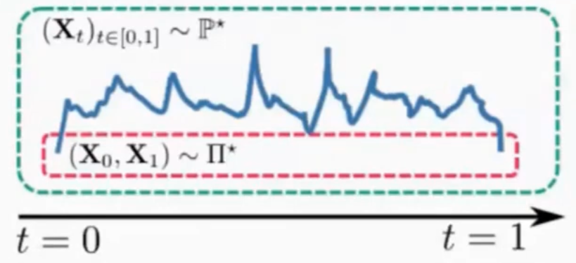
The dynamic formulation is what Schrödinger formulated back in the 1930s, without even having the right “language” at the time
where $\mathbb{Q}$ is a reference path measure, for instance some scaled Brownian motion \((\sqrt{\varepsilon} \mathbf{B}_t)_{t\in[0,1]}\). The path measure $\mathbb{P}^*$ is called a Schrödinger bridge and can be thought of a path measure closest to $\mathbb{q}$ in distribution which satisfies the marginal constraints $\mathbb{P}_0 = \pi_0$ and $\mathbb{P}_1 = \pi_1$
Conclusions
The Schrödinger Bridge problem elegantly connects several fundamental concepts in mathematics and machine learning. What started as Schrödinger’s attempts to understand quantum mechanics in the 1930s has evolved into a powerful framework bridging optimal transport, statistical physics, and information theory, with applications reaching far beyond physics, such as machine learning and even economics.
The dynamic formulation of optimal transport, as opposed to the static one, provides a key insight into why modern generative models like diffusion models work so well. Instead of trying to learn a one-shot mapping between distributions (GANs, VAEs), they break down the transportation problem into a sequence of smaller steps, which allows iteratively refining the samples over many stages.